Training a Convolutional Neural Network in the Browser

Introduction to Convolutional Neural Networks (CNNs)

Convolutional Neural Networks (CNNs) are a class of deep learning models widely used for analyzing visual imagery, such as images or videos. CNNs use convolutional layers that automatically learn spatial hierarchies of features from input images, making them highly effective for image classification, object detection, and related tasks. A typical CNN architecture consists of convolutional layers, pooling layers, and fully connected layers.

• Convolutional Layers: Apply filters to extract features like edges, textures, and shapes.
• Pooling Layers: Reduce the spatial dimensions, retaining the most important information.
• Fully Connected Layers: Perform classification based on the extracted features.

Training a CNN involves feeding labeled images into the model, computing the loss between predictions and ground truth, and updating the model's weights using backpropagation and optimization algorithms (commonly stochastic gradient descent or Adam).

Training a CNN

To train a CNN, you need:

• A dataset of labeled images (e.g., MNIST for handwritten digit recognition).
• A defined CNN architecture (number of layers, filter sizes, activation functions, etc.).
• A loss function (e.g., categorical crossentropy for classification tasks).
• An optimizer (e.g., Adam or SGD).

Visualizing a CNN Structure

Easy-to-Understand Example

Imagine teaching a computer to recognize handwritten numbers, like distinguishing a '5' from a '3'. Here’s how a CNN learns this task:

1. Input: The CNN receives an image of a handwritten digit (for example, a 28x28 pixel grayscale image).
2. Convolution: The first layer applies small filters that scan the image, detecting simple patterns like lines and curves.
3. Pooling: The next layer reduces the size of the data, keeping only the most important information.
4. Flatten & Dense: The condensed information is flattened into a vector and passed through fully connected ("dense") layers, which learn to associate patterns with specific digits.
5. Output: The network outputs the probability for each digit (0-9). The highest probability is the model's guess.

With enough training examples, the CNN learns which patterns correspond to each digit, just like how you learned to recognize handwriting!

TensorFlow.js for CNN Training in JavaScript

TensorFlow.js is a JavaScript library for training and deploying machine learning models in the browser or Node.js. It allows you to define, train, and run neural networks entirely in JavaScript, leveraging GPU acceleration via WebGL.

• Model Definition: Use tf.sequential() or tf.model() to construct models.
• Layers: Use tf.layers.conv2d(), tf.layers.maxPooling2d(), and tf.layers.dense() for CNN architectures.
• Training: Call model.compile() to set the optimizer and loss, and model.fit() to train the network.
• Data: You can use built-in datasets, load images, or use data generated in the browser.

TensorFlow.js enables real-time model training and inference directly in the browser, making it ideal for interactive machine learning demos and educational purposes.

Try it: Train a Simple CNN on MNIST Digits

The demo below will automatically download a sample of the MNIST dataset, define a small CNN, and train it right in your browser.

Libraries for Model Definition, Training, and Visualization

Several JavaScript libraries are available to help you define, train, and visualize neural network models in the browser:

• TensorFlow.js — An open-source library for defining, training, and running machine learning models entirely in the browser using JavaScript.
  https://cdn.jsdelivr.net/npm/@tensorflow/tfjs@1.7.4/dist/tf.min.js
• Plotly.js — A high-level, interactive charting library for visualizing data and model training progress directly on web pages.
  https://cdn.jsdelivr.net/npm/plotly.js@1.54.7/dist/plotly.min.js

These libraries can be used together to build, train, and visualize neural network models directly in your web browser.

Discussion: The MNIST Image Dataset and Labels

The MNIST dataset is a classic benchmark in machine learning, featuring grayscale images of handwritten digits (0 through 9). Each image is 28x28 pixels (784 total), and the goal is to train a model to recognize the digit each image represents.

• Image File: mnist_images.png
  This single PNG image contains 65,000 stacked digit images in row-major order (each row is a 28x28 square).
• Labels File: mnist_labels_uint8
  This binary file contains the digit label (0–9) for each image, stored as unsigned 8-bit integers.

These files are commonly used for training and evaluating image classification models. By pairing images with their correct labels, we can teach a neural network to recognize handwritten digits.

Visualize MNIST Data Samples

Now that the dataset cleanedData is loaded, you can browse and visualize any digit and its label below. Use the input to select an index (from 0 to ?).

Splitting the Dataset into Training and Testing Sets

In machine learning, it is important to divide your dataset into two separate parts: a training set and a testing set. The training set is used to train the model, while the testing set is used to evaluate its performance on unseen data. A common split is 80% for training and 20% for testing, but the ratio can be adjusted as needed. This helps ensure the model generalizes well and does not simply memorize the examples.

Defining a Convolutional Neural Network (CNN) Model

Now that the data is ready, let's define a Convolutional Neural Network (CNN) model in JavaScript using TensorFlow.js. CNNs are especially effective for image recognition tasks such as classifying handwritten digits from the MNIST dataset.

Understanding the CNN Model

The Convolutional Neural Network (CNN) is designed for image recognition. It works in several steps:

1. Convolution: Learns small patterns (like edges or curves) in the image using sliding "filters".
2. Pooling: Reduces the size of the image while keeping important information, helping the model to focus on major features.
3. Dense (Fully Connected) Layers: These combine patterns detected in earlier layers to make the final prediction.

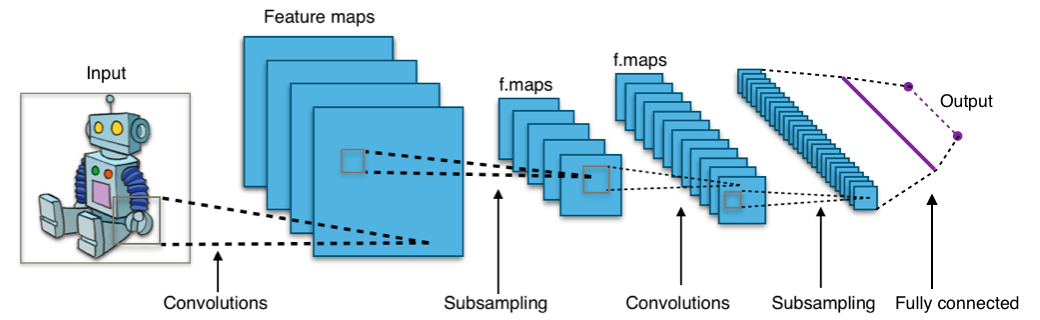
Here’s an illustration of how a CNN processes an image:

• Left: Input image (28x28 pixels)
• Middle: Filters detect features (edges, shapes)
• Right: Final layers combine features for classification

Animation and more interactive visualizations of CNNs can be found on CNN Explainer.

Training the CNN Model

Now that the CNN model is defined, the next step is to train it using the training dataset. During training, the model learns to recognize patterns in the data by adjusting its internal weights to minimize prediction errors. This is done over multiple cycles called epochs. After each epoch, the model's performance on the training data is measured by loss (error) and accuracy (correct predictions).

How Model Training Works

Training is the process where the model learns by comparing its predictions to the known correct answers in the training data. The model adjusts its internal settings (weights and biases) to make better predictions. This cycle repeats for multiple epochs to gradually improve accuracy.

Above: Each training epoch moves the model's predictions closer to the correct result, like stepping down a hill to reach the lowest point (minimal error).

Testing the CNN Model

After training, it's important to evaluate how well the model performs on unseen data. This is called testing the model. Testing uses a separate portion of the dataset that was not used during training. It helps determine if the model has learned general patterns or just memorized the training data.

How Model Testing Works

During testing, the model makes predictions on new data it has never seen before. The results are compared to the actual labels to calculate loss (how far off the predictions are) and accuracy (how often it gets the right answer). High accuracy and low loss on the test set mean the model can generalize well to real-world data.

Above: Evaluating a model involves measuring how often it makes correct predictions on new, unseen data.

Understanding the Confusion Matrix

The confusion matrix is a table used to describe the performance of a classification model on a set of data for which the true values are known. It shows how many predictions were correct and where errors occurred, breaking down predictions by each class. The matrix helps you identify if the model is confusing certain classes, and is especially useful for multi-class problems like digit recognition.

• Rows: Actual labels (ground truth)
• Columns: Predicted labels by the model
• The main diagonal shows correct predictions, while off-diagonal values indicate misclassifications.

How to Interpret the Confusion Matrix

The confusion matrix helps you see which classes the model is predicting well and where it makes mistakes. For example, if many actual "3"s are misclassified as "5", you'll see a higher count in the row for "Actual 3" and the column for "Pred 5".

Diagonal cells are correct predictions. Off-diagonal cells represent mistakes and reveal which classes the model confuses.